Plot GMM Entropy Class Trajectory for a Single Site

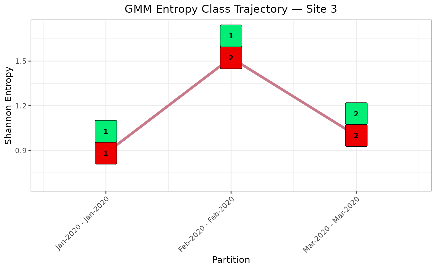
Plots the Shannon entropy trajectory for a single sequence site across time partitions, with geom-label overlays at each partition recording the site's current GMM class (above the line, in green) and the partition's highest-entropy class label (below the line, in red). The visual contrast between the two labels tracks the moment a site enters the highest-entropy cluster — the entropy-based analogue of variant emergence detection.

Usage

plot_site_class_trajectory(
  data_frame,
  site,
  site_color = "steelblue",
  xbreaks,
  xlabels,
  col_current = "springgreen2",
  col_max_class = "red2",
  label_size = 3,
  x_angle = 45,
  line_size = 1.5,
  plot_title = NULL,
  save = FALSE,
  save_path = NULL,
  save_extension = ".png",
  width = 20,
  height = 15,
  dpi = 300
)

Arguments

data_frame: Data frame. The $Data_Frame element from plot_entropy_trajectories. Must contain columns sites, entropies, class, max_class, period, and coverage.
site: Integer (length 1). The site index to plot. Must be present in data_frame$sites.
site_color: Character. Colour of the entropy trajectory line. Default is "steelblue". Pass plot_entropy_trajectories()$Colors[as.character(site)] for cross-plot colour consistency.
xbreaks: Integer vector. Partition period indices for x-axis breaks. Typically plot_entropy_trajectories()$XBreaks.
xlabels: Character vector. Partition label strings aligned with xbreaks. Typically plot_entropy_trajectories()$XLabels.
col_current: Character. Fill colour of the upper geom-label (current GMM class at each partition). Default is "springgreen2".
col_max_class: Character. Fill colour of the lower geom-label (highest-entropy class label at each partition). Default is "red2".
label_size: Numeric. Font size of the class integer text inside the geom-labels. Default is 3.
x_angle: Numeric. Rotation angle of x-axis tick labels in degrees. Default is 45.
line_size: Numeric. Width of the entropy trajectory line. Default is 1.5.
plot_title: Character or NULL. Plot title. If NULL (default), the title is auto-generated as "GMM Entropy Class Trajectory \u2014 Site <site>".
save: Logical. If TRUE, the plot is saved to disk via ggsave. Default is FALSE.
save_path: Character or NULL. Directory in which to save the file. Created recursively if it does not exist. Must be supplied when save = TRUE. Default is NULL.
save_extension: Character. File extension including the leading dot (e.g. ".jpeg", ".pdf", ".png"). Default is ".jpeg".
width: Numeric. Saved figure width in inches. Default is 20.
height: Numeric. Saved figure height in inches. Default is 15.
dpi: Numeric. Resolution of the saved raster output in dots per inch. Default is 600.

Value

A ggplot object (returned invisibly). Additional ggplot2 layers can be appended with + before printing or saving, for example:


p <- plot_site_class_trajectory(traj$Data_Frame, site = 681L, ...)
p + ggplot2::geom_vline(xintercept = 14, colour = "darkorange",
                         linetype = "dashed", linewidth = 1.5)

Details

The function operates on the $Data_Frame element returned by plot_entropy_trajectories, which contains columns sites, entropies, class, max_class, period, and coverage.

Class label interpretation. The green label (upper) records the GMM class assigned to the site in that partition; the red label (lower) records max_class — the label of the highest-entropy component for that partition. When the two labels are equal the site has entered the highest-entropy class. Without relabeling, max_class is the raw Mclust label carrying the highest mean entropy (i.e. max(classification) at clustering time). When the user has pre-relabeled the partitions via relabel_entropy_classes before calling plot_entropy_trajectories, max_class is 1L throughout (class 1 is the highest-entropy group by definition), and the sentinel 999L is preserved unchanged.

Axis padding. Both axes carry generous expansion margins so that geom-label boxes at extreme entropy values or at the first and last partitions do not clip the panel border. The returned ggplot object can be further adjusted by appending standard ggplot2 layers with + before printing or saving.

Examples

# Three-period synthetic dataset (independent of plot_entropy_trajectories'
# example). Three sites with different entropy trajectories; site 1 features
# a monotone-up trajectory and progressively higher rank among sites,
# producing class changes across all three partitions.
#
# Site 1 follows a monotone-up trajectory (0.469 -> 0.881 -> 1.522), 
# climbing from lowest rank in P1 to highest in P3 for a clear 
# "emerging variant" class progression. Site 2 follows the
# opposite trajectory (1.522 -> 1.000 -> 0.881), starting as the dominant
# high-entropy site and declining as site 1 rises. Site 3 (featured) 
# peaks at P2 (0.881 -> 1.522 -> 1.000).
#
# Per-partition Shannon entropy (bits):
#          P1     P2     P3
#   s1   0.469  0.881  1.522   
#   s2   1.522  1.000  0.881
#   s3   0.881  1.522  1.000   <- featured site
df_cls <- data.frame(
  s1 = c(
    c(1L, 1L, 1L, 1L, 1L, 1L, 1L, 1L, 1L, 2L),       # P1: 9:1
    c(1L, 1L, 1L, 1L, 1L, 1L, 1L, 2L, 2L, 2L),       # P2: 7:3
    c(1L, 1L, 1L, 1L, 2L, 2L, 2L, 2L, 3L, 3L)        # P3: 4:4:2
  ),
  s2 = c(
    c(1L, 1L, 1L, 1L, 2L, 2L, 2L, 2L, 3L, 3L),       # P1: 4:4:2
    c(1L, 1L, 1L, 1L, 1L, 2L, 2L, 2L, 2L, 2L),       # P2: 5:5
    c(1L, 1L, 1L, 1L, 1L, 1L, 1L, 2L, 2L, 2L)        # P3: 7:3
  ),
  s3 = c(
    c(1L, 1L, 1L, 1L, 1L, 1L, 1L, 2L, 2L, 2L),       # P1: 7:3
    c(1L, 1L, 1L, 1L, 2L, 2L, 2L, 2L, 3L, 3L),       # P2: 4:4:2
    c(1L, 1L, 1L, 1L, 1L, 2L, 2L, 2L, 2L, 2L)        # P3: 5:5
  ),
  Date = rep(
    seq(as.Date("2020-01-01"), by = "month", length.out = 3L),
    each = 10L
  )
)

part_data <- partition_time_windows(
  data          = df_cls,
  n_sites       = 3L,
  window_length = 1L,
  window_type   = 3L,
  start_date    = "2020-01-01",
  end_date      = "2020-04-01",
  removez       = FALSE,
  removesngl    = FALSE
)

# Apply class relabeling so class 1 = highest mean entropy.
# plot_entropy_trajectories does not relabel internally; the consumer does.
for (i in seq_along(part_data$Clusters)) {
  part_data$Clusters[[i]]$DataFrame <-
    relabel_entropy_classes(part_data$Clusters[[i]]$DataFrame)
}

traj <- plot_entropy_trajectories(part_data)

p <- plot_site_class_trajectory(
  data_frame = traj$Data_Frame,
  site       = 3L,
  site_color = traj$Colors["1"],
  xbreaks    = traj$XBreaks,
  xlabels    = traj$XLabels
)
print(p)

Usage

Arguments

Value

Details

See also

Examples